Administrivia
This article was initially posted on Wikipedia in 2008, which explains why it's written at the 3rd person and looks familiar to articles on binary trees. A few moderators decided that the article was only self-promotion and removed it without notification a few days after its publication. After many arguments with them, I was told that Wikipedia cannot hold original work, only copies of what can be found somewhere else, and I gave up the fight, realizing that for once I found dumber than me! At least they accepted to let me retrieve the original work so that I can publish it somewhere else (I didn't even have a copy of it). Needless to say I have stopped donating to Wikipedia since then. Three years later, I spent part of a week-end putting this online here. When I have time, I'll rewrite it differently.Introduction
In computer science, an elastic binary tree (or EB tree or EBtree) is a binary search tree specially optimized to very frequently store, retrieve and delete discrete integer or binary data without having to deal with memory allocation. It is particularly well suited for operating system schedulers where fast time-ordering and priority-ordering are strong requirements. Insertion and lookups are performed in O(log n) while removal is done in O(1). The tree is not balanced but its height is bound by the type of data to store in it. Ordered duplicate entries are also natively supported.The elastic binary tree was invented between 2002 and 2007 by Willy Tarreau as part of a research work on an event-based task scheduler for user-space network applications. This type of components require a sorted list of future events, and insertion and removal are very common operations which must be optimized. An early implementation relied on a naive linked list approach, soon replaced with a fast radix tree. The disadvantages of the radix tree is that it is often necessary to allocate memory for one node to store a value, and that some garbage collection must be performed after removal in order to eliminate unused nodes. There are situations where this is not desirable nor even possible. An alternative was to use a balanced tree, but the very frequent removal operation costs O(log n).
The solution was to find some sort of hybrid type of tree between both, where each inserted entry would carry both an intermediate nodes and a leaf, both of which would stray from each other as the tree leaves, thus stretching the initial node across levels, hence the name "elastic binary tree".
License
The concept and algorithms have been released under public domain. The author's implementation was first released under GPL then switched to LGPL for more openness. The algorithm is simple enough to allow other implementations to be initiated for very specific needs.Definitions
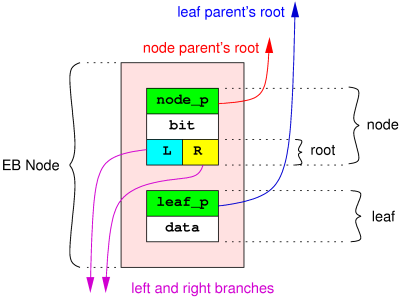 In an EB tree, data are stored in EB nodes. An EB node contains two parts :
 - the node part, which is responsible for tying together upper and lower nodes or leaves ;
- the leaf part, which carries the data (an integer key), and keeps a pointer to its upper node (leaf_p).
The node part itself is composed of a parent pointer (node_p), a level (bit), and a root, which itself links to lower nodes constituting a subtree.
The level part represents the lowest bit position in the key, above which all bits are equal for all keys in the lower subtrees.
A root only contains two links called branches, which represent the value of the bit below current node's. There is always a left and a right branch, except for the top of the tree. Left branch represents bit value 0 while right branch reprensents value 1.
Branches are typed. This means that a node knows whether its branches point to other nodes or to leaves. Parent pointers are typed too. This means that each node or leaf knows if it is attached to the left or the right branches of the upper root.
A typical EB tree begins with a root at its head, containing 0 or 1 branch, below which the tree is complete. The right branch of an EB tree root is always empty.
Features
EB trees offer a wide range of useful data manipulation features :- Lookup :
- lookup first or last key
- exact match: lookup exact key (signed/unsigned integer, poitner, string or memory block)
- longest match: lookup longest matching key (network address match)
- lookup first matching prefix: retrieve first entry matching the beginning of a key
- lookup closest smaller value
- lookup closest greater value
- lookup previous or next different value: quickly skip duplicates
- lookups of duplicate keys always performed in key insertion order
- Insertion :
- standard key insertion : if the key exists, create a duplicate entry
- unique key insertion : if the key exists, return the existing one
Complexity
EB trees algorithmic complexity can be derived from 3 variables :- the number of possible different keys in the tree : P
- the number of entries in the tree : N
- the number of duplicates for one key : D
Minimal, Maximal and Average times are specified in number of operations. Minimal is given for best condition, maximal for worst condition, and the average is reported for a tree containing random keys. An operation generally consists in jumping from one node to another.
Complexity :
- lookup : min=1, max=log(P), avg=log(N)
- insertion from root : min=1, max=log(P), avg=log(N)
- insertion of dups : min=1, max=log(D), avg=log(D)/2 after lookup
- deletion : min=1, max=1, avg=1
- prev/next : min=1, max=log(P), avg=2 :
 N/2 nodes need 1 hop=> 1*N/2
 N/4 nodes need 2 hops => 2*N/4
 N/8 nodes need 3 hops => 3*N/8
 ...
 N/x nodes need log(x) hops => log2(x)*N/x
 Total cost for all N nodes : sum[i=1..N](log2(i)*N/i) = N*sum[i=1..N](log2(i)/i)
 Average cost across N nodes = total / N = sum[i=1..N](log2(i)/i) = 2
Current EB tree design is limited to only two branches per node. Most of the tree descent algorithm would be compatible with more branches (eg: 4, to cut the height in half), but this would probably require more complex operations and the deletion algorithm would be problematic.
Properties
EB trees have several useful properties :- a node is always added above the leaf it is tied to, and never can get below nor in another branch. This implies that leaves directly attached to the root do not use their node part, which is indicated by a NULL value in node_p. This also enhances the cache efficiency when walking down the tree, because when the leaf is reached, its node part will already have been visited (unless it's the first leaf in the tree).
- pointers to lower nodes or leaves are stored in "branch" pointers. Only the root node may have a NULL in either branch, it is not possible for other branches. Since the nodes are attached to the left branch of the root, it is not possible to see a NULL left branch when walking up a tree. Thus, an empty tree is immediately identified by a NULL left branch at the root. Conversely, the one and only way to identify the root node is to check that it right branch is NULL. Note that the NULL pointer may have a few low-order bits set on some implementations.
- a node connected to its own leaf will have one and only one of its branches pointing to itself, and leaf_p pointing to itself.
- a node can never have node_p pointing to itself.
- a node is linked in a tree if and only if it has a non-null leaf_p.
- a node can never have both branches equal, except for the root which can have them both NULL.
- deletion only applies to leaves. When a leaf is deleted, its parent must be released too (unless it's the root), and its sibling must attach to the grand-parent, replacing the parent. Also, when a leaf is deleted, the node tied to this leaf will be removed and must be released too. If this node is different from the leaf's parent, the freshly released leaf's parent will be used to replace the node which must go. A released node will never be used anymore, so there's no point in tracking it.
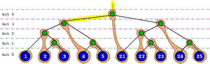
- the bit index in a node indicates the bit position in the key which is represented by the branches. That means that a node with (bit == 0) is just above two leaves. Negative bit values are used to build a duplicate tree. The first node above two identical leaves gets (bit == -1). This value logarithmically decreases as the duplicate tree grows. During duplicate insertion, a node is inserted above the highest bit value (the lowest absolute value) in the tree during the right-sided walk. If bit -1 is not encountered (highest < -1), we insert above last leaf. Otherwise, we insert above the node with the highest value which was not equal to the one of its parent + 1.
- the "eb_next" primitive walks from left to right, which means from lower to higher keys. It returns duplicates in the order they were inserted. The "eb_first" primitive returns the left-most entry.
- the "eb_prev" primitive walks from right to left, which means from higher to lower keys. It returns duplicates in the opposite order they were inserted. The "eb_last" primitive returns the right-most entry.
- a tree which has 1 in the lower bit of its root's right branch is a tree with unique nodes. This means that when a node is inserted with a key which already exists will not be inserted, and the previous entry will be returned.
Principles of operations
Insertion
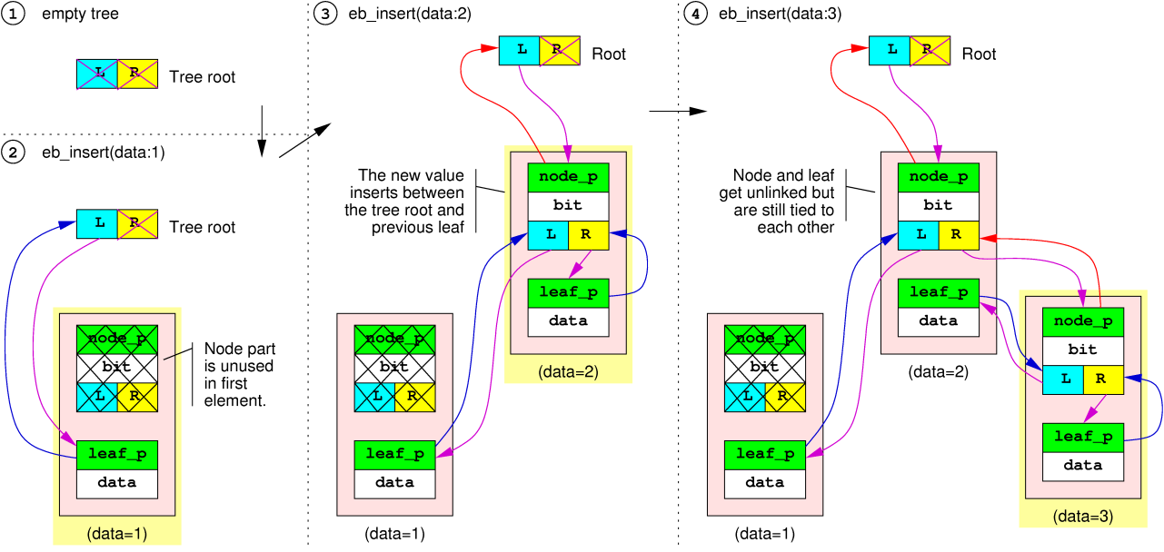
Initially, a tree is empty. It only consists in a root with two NULL pointers (one for each branch).
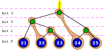
When the first EB node is inserted, its leaf is directly linked to the root 's left branch. Thus, its node part is not used. It is the only situation where a node part is not used. After that, a new EB node is inserted. A node part is needed between the root and existing leaf to connect the new leaf. This is where the node part provided with the new EB node will be used. The second EB node's node part will have one of its branch pointing to the previous leaf, and the other branch pointing to its own leaf. For this reason, it is not possible to have an empty branch below a node.
When the third EB node is added, it may very well insert itself between the node and the leaf of previous EB node, which will be stretched by the operation. It is important to note that the node part of a stretched EB node is always located somewhere between the root and the leaf of the same EB node. The same principle goes on with further keys, as shown on the diagrams below.
|
|

Insertion of duplicates
An EB tree supports duplicates and keeps them ordered. This is a very important property for a fair scheduler because events stored with the same wake-up date must be processed in the same sequence to avoid risks of starvation.In order to store a duplicate key, we grow a binary sub-tree at the place where the leaf was to be located, using the same algorithm as for the upper tree, but with negative bit offsets. This allows duplicates to be stored without overhead data, and to be walked through using the same functions, without any processing overhead. The nodes order is respected and all nodes will be walked in their insertion order.
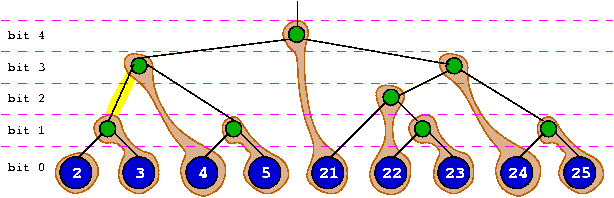
Deletion
When a leaf is deleted, its parent must be released too (unless it's the root), and its sibling must attach to the grand-parent, replacing the parent. Also, when a leaf is deleted, the node tied to this leaf will be removed and must be released too. If this node is different from the leaf's parent, the freshly released leaf's parent will be used to replace the node which must go. EB trees do not need to be rebalanced after deletion. This results in tree deletion being performed in O(1). A released node will never be used anymore, so there's no point in tracking it.
|
|
Tree walk
A tree walk may be performed from left to right or right to left, always following numerical order and duplicates insertion order if applicable. It relies on the following primitives :- eb_first(root): return the first node of the tree starting at [root]
- eb_last(root): return the last node of the tree starting at [root]
- eb_next(node): return next node after [node]
- eb_prev(node): return previous node before [node]
- eb_next_unique(node) : return the next node with a different key from current [node].
- eb_prev_unique(node) : return the previous node with a different key from current [node].
Implementation specifics
The only currently known implementation is the author's. It works on 32- and 64-bit platforms, either little or big endian. It uses the fact that pointer storage is 32-bit aligned at least, causing structure pointers to always have their two lowest bits cleared. This allows for pointer type to be stored in the pointer itself :- a node pointer will be stored verbatim (with lowest bit cleared)
- a leaf pointer will be stored with lowest bit set (which equals pointer + 1)
- a parent pointer in a left branch will be stored verbatim (with lowest bit cleared)
- a parent pointer in a right branch will be stored with lowest bit set (which equals pointer + 1)
The right branch of the root must always be NULL. However, applying the same principle as above lets us put global flags in this location. Currently, the only used flag is EB_ROOT_UNIQUE, indicated by setting the lowest bit of the right branch pointer in the root. It indicates that duplicates are not desired and that when a key already exists during an insertion, nothing may be inserted and the existing node will be returned instead.
The current implementation is split between generic code and type-specific code. This makes it easier to later add support for newer types. Currently, pointers, signed/ unsigned 32/64 bit integers, strings and arbitrary memory blocks are supported.
Sixth version of the author's implementation brought support for prefix-based matching of memory blocks, which supports prefix insertion and longest match which are still compatible with the rest of the common features (walk, duplicates, delete, ...). This is typically used for network address matching or route selection. This update is not (yet) covered by this document.
Seventh version of the author's implementation brings support for a remappable variant of the ebtree called rebtree (rremappable elastic binary tree). This version is slightly slower but works on relative pointers, making it suitable for use in mapped files.
The current implementation distinguishes between eb_node which is type-agnostic and ebXX_nodewhich is a node of type XX. In practise, an eb_node has everything except the key itself. Only insertion and lookup need the key, all other operations only operate on the structure of the tree. This allows most primitives to be shared between type-specific implementations :
/* generic types */
typedef void eb_troot_t;

struct eb_root {
 eb_troot_t*b[EB_NODE_BRANCHES]; /* left and right branches */
};

struct eb_node {
 struct eb_root branches; /* branches, must be at the beginning */
 eb_troot_t*node_p; /* link node's parent */
 eb_troot_t*leaf_p; /* leaf node's parent */
 int bit; /* link's bit position. */
};

/* 32-bit specific types */
typedef unsigned int u32;

struct eb32_node {
 struct eb_node node; /* the tree node, must be at the beginning */
 u32 key;
};
The structures were designed to be located at the very beginning of any structure making use of EB trees. It is important for cache efficiency and memory access time that the EB tree data are located at the beginning of a CPU cache line, especially the 4 first pointers.
Performance considerations
The author uses EB trees in areas where red-black trees were burning too many CPU cycles. The haproxy load balancer has switched to EB trees and shows minor CPU usage at speeds up to 500000 insertions/removals per second, and a firewall log analyser relies on it to sort logs at speeds above one million lines per second. An insertion typically takes less than 100 nanoseconds on modern machines.EB trees are much faster than conventional balanced trees when looking up strings or memory blocks because during the tree descent, only the bits specific to the new node are compared, while in a balanced tree, the string compare has to be performed on the whole string for each step. This advantage is emphasized in the halog log analyser which is able to process more than 4 million lines per second while indexing URLs.
The ability to lookup prefixes has made EB trees able to perform an operation which previously was possible only in radix trees but not in binary trees. Having the ability to use the same tree for various purposes can sensibly reduce complexity in some implementations, and reduce the number of operations (eg: network routing and filtering). Tests have shown that network lookups within a BGP table containing 450000 routes could be performed several million times a second on a modern machine.
However, a tree node is typically 20-bytes long on a 32-bit system. On systems with very small caches or low memory bandwidth, EB trees can be slower than red-black trees if insertions/removals are not much frequent and do not compensate for the increased bandwidth usage. Also, red-black trees rely on the ability to compare values, which make them suitable for many data types. Conversely, EB trees heavily rely on bit-addressable data (typically integers), which confer them a very high performance due to the cheap operations involved, but limit their application field. Trying to use EB trees to store non-bit-adressable data would completely defeat their purpose and will likely provide poor performance.
Practical uses
The HAProxy load balancer uses EB trees for the following features :- timers: timers are stored ordered, which ensures that checks for timeouts are always performed in O(1).
- scheduler: the scheduler maintains the list of runnable tasks by weighting their wake-up order with their nice value. EB trees make this operation very cheap, typically O(Log(N)), allowing priorities to be used with huge amounts of tasks without any noticeable cost.
- ACL: string and IP address matches rely on EB trees so that even very large pattern file do not cause any noticeable slowdown (eg: full internet BGP routing table).
- stick-tables: data learned from traffic (cookies, SSL ID, headers, URLs, ...) are stored and retrieved using EB trees
- The multi-peer sync protocol uses the ability to lookup ranges in EB trees.
The halog log analyser provided with HAProxy uses EB trees to sort counters, stats, URLs and servers.
The Scalable TLS Unwrapping Daemon (stud) uses EB trees for its shared session cache.
At least one proprietary log analysis solution makes extensive use of the remappable version of the EB trees for fast log indexing and lookup.
At least one thread-safe variant is known to exist, though very little is known about it at this time.
It is not very clear how this is better than the radix tree. Please elaborate on that. Why would the allocations and deletions be lesser here?
ReplyDeleteWith a normal radix tree, the allocation will depend on whether the value you want to add already exists or not. Each node will typically be a list head to which you attach all nodes having an identical value. Depending on how your radix tree is built, you may even have to allocate the intermediary nodes and the leaf nodes separately. Here the approach is different, you allocate one item which contains both the node and the leaf, and you can use these two parts to plug it anywhere into an existing tree, even supporting duplicated values if needed.
ReplyDeleteAre there any benchmarking studies? I stumbled on this recently. I am especially interested n the longest prefix matching applications.
ReplyDeleteNot that I'm aware. I used to do some against rbtrees during development a long time ago, and the outcome was that we removed rbtrees from haproxy's scheduler which now uses ebtrees instead. For a scheduler, nodes are inserted once, removed once, and visited only once via a next() operation. Thus, switching from O(logN) to O(1) for removal basically cuts the cost in half. For some keys like timers, prefix trees are very interesting because they tend to group objects that are visited at the same moment, so most of the visited nodes during the tree descent for an insertion are hot in the cache at the same time. For the longest prefix match, I suggest that you have a look at examples/reduce.c which merges overlapping networks and produces a more compact list, and/or to pat_match_ip() in haproxy, which we use for both IPv4 and IPv6.
DeleteThank you for the pointers. I will look at those.
Delete